Introduction

With the widespread adoption of engineering software and computerized design processes, it is commonly thought that engineering calculations are very accurate. However, while engineering software can eliminate mathematical errors and perform calculations with greater speed than hand calculations, there are many factors that must be acknowledged which can result in the calculated values being substantially different from actual measurements. This article will discuss some of the factors that can make calculations vary from measured results, including factors related to system construction as well as to system modeling. These factors can then be considered during system design to ensure that the design will meet all necessary requirements. In addition, consideration of these factors is also prudent when troubleshooting existing systems to avoid drawing unwarranted or incorrect conclusions.

Construction Issues

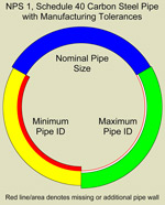
When analyzing fluid flow problems, the designer typically uses nominal dimensions for pipe and fittings. A nominal dimension is similar to an average dimension. No specific pipe or fitting is guaranteed to match the nominal dimensions exactly. Consider a nominal NPS 1, schedule 40 carbon steel pipe dimensioned using ANSI B36.10, Welded and Seamless Wrought Steel Pipe and constructed to ASTM A 106 - 91, Standard Specification for Seamless Carbon Steel Pipe for High-Temperature Service. These are common specifications for carbon steel pipe. For this nominal pipe, the nominal inside diameter is 1.049 inches. The material specification imposes limits on variation in dimensions, including limits on the pipe outside diameter, limits on the pipe wall thickness, and limits on the pipe weight. According to these limits, this pipe could have an inside diameter as large as 1.079 inches or as small as 0.978 inches (localized measurements could even be outside this range). These as-built dimensions could result in a calculated head loss from 13.7 percent under to as much as 44.6 percent over the calculated head loss for the nominal pipe (both calculated with the same volumetric flow rate and with fully turbulent flow). Similarly for a large pipe such as a NPS 24, schedule 20 to the same specifications, the calculated head loss could range from 3.4 percent under to 2.5 percent over the nominal head loss. In general, this potential error is larger for smaller diameter pipe, larger nominal wall thickness, and higher flow rates.

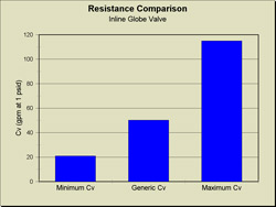
Similarly, for items other than pipe, most analyses use resistance values based on generic items. For example, many sources provide a resistance value for an inline globe valve equal to 340 diameters of pipe. (Some sources are slightly different, but this doesn’t change the conclusion). This resistance value is combined with a turbulent friction factor for the appropriate size to calculate the resistance of the valve. When you compare this resistance for a generic valve to actual manufacturer data, there can be considerable differences. For example, comparing the resistance of a generic, 2 inch inline globe valve to a small sample of commercially available valves shows that the resistance of the generic valve can be as much as 38 percent under to 25 percent over that of the commercial valve which would result in an identical variation in head loss at a constant flow. This difference is caused largely because different valves are designed for different characteristics, such as good throttling or low resistance, and are not truly represented by a single generic value. In general, where data is available for a specific valve or fitting, this data should be used instead of the generic information.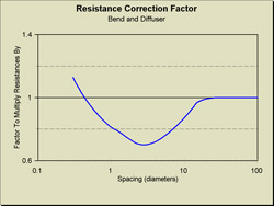

Further, the resistance of a fitting is generally determined in isolation, meaning that a single fitting is placed between two long sections of pipe and the flow and head loss are measured. If fittings in a system are not separated sufficiently, then the head loss produced by each fitting can differ from that of an isolated component (the normal resistance for that component). While there is no formula for calculating the effect and this difference has not been quantified for all arbitrary combination of fittings and spacing, it has been measured for simple combinations such as two 90 degree bends separated by small lengths of straight pipe. With two bends, the use of normal resistance values determined in isolation can overstate the actual resistance by as much as 50 percent or understate the resistance by 300 percent. The actual resistance of two closely spaced bends depends on the specific type of bends (including factors such as the bend type, angle, and radius), the orientation of the bends, and the spacing between the bends. This is even more complex for other combinations of fittings, and currently no general method exists to calculate modified resistance values. In general, however, the use of an isolated resistance value generally (but not always) overstates the actual resistance of the item.

Modeling Issues

A common way of expressing resistance of an item is with a dimensionless factor denoted ‘K’. If a fitting has the same geometry for different sizes, the K factor for the fitting will be the same for each size. However, the geometry of fittings is generally different for each different size (in other words, it does not change proportionally with size). Consequently, common practice is to represent the resistance of a fitting as the number of diameters of straight pipe that would cause the same pressure drop (generally denoted ‘L/D’). This number is generally the same for different sizes of a given fittings. This value is then combined with the turbulent friction factor for the size of the fitting to obtain a resistance value.

This assumption to use a turbulent friction factor is based on extensive testing and has been shown to be valid down to small flow rates. In the case of a simple bend, the assumption of a turbulent friction factor is valid down to a Reynolds number of less than 500. For other fittings, with more extreme changes in flow direction or flow area, it would be expected that this assumption would hold at even lower Reynolds numbers. However, beyond this value, the resistance of the item can increase substantially (in the case of a simple bend by a factor of over 100 compared to the turbulent value at a Reynolds number of 10).

Pipes on the other hand are always analyzed with a friction factor determined based on the actual flow rate and internal surface condition. In most cases, the internal surface of the pipe will become rougher with age, resulting in increased head loss compared to new pipe. Analysis for a large water distribution system showed increases in head loss through cast iron pipe of up to 800% over 40 years. Other studies with steel pipe have shown smaller but still significant increases, with increases in head loss ranging from 40% to 200% over 20 years.

Beyond the issue of what roughness to use, and what friction factors are appropriate, there is still the issue of the accuracy of the head loss equations themselves. There are several to choose from, including empirical relationships such as the Hazen-Williams formula for liquids, and the Panhandle and Weymouth formulas for gases. However, because of its range of applicability and overall accuracy, for liquids the Darcy-Weisbach equation is generally used. First proposed in this form in 1845 by Julies Weisbach, this equation relates head loss through pipe to the square of the average fluid velocity in the pipe. The current form of this equation is routinely called the Darcy equation, after Henry Darcy, who made significant achievements in understanding and documenting the friction factor and its relationship to the pipe inside surface condition. This equation is also commonly used for valves and fittings in addition to pipe. However, experiments have shown that while the Darcy equation is a practical solution method for valves and fittings, actual flow measurements have shown that the head loss for any given valve or fitting design is proportional to velocity raised to an exponent of between 1.8 to 2.1 instead of the exponent of 2 assumed in the Darcy equation. Nonetheless, common practice is to use the Darcy equation unmodified for valves and fittings.

Conclusion

The factors discussed here are generally applicable to all fluid flow problems. However, for an individual problem these factors may or may not be significant in the context of the whole problem. When performing a fluid flow calculations, an engineer should review these factors and determine what, if any, actions should be taken to accommodate the uncertainty they introduce. In general, actions taken by an engineer may include performing additional analysis (such as calculations with different pipe diameters or with different pipe roughness), adding additional margin to a design, or performing actual tests on as-built systems.